Database Math – Database mathematics and more pragmatic information.

MSSQL 2016/2017 to 2019 Upgrade with Polybase installed – Switching from Oracle JRE to Azul Open JDK JRE

How to change from Oracle Java JRE to Azul Open JRE for Polybase when upgrading from SQL Server 2016/2017 to 2019

Background:

The Polybase feature was first introduced in SQL Server 2016. The data virtualization solution enabling customers to query data in Cloudera or Hortonworks from SQL Server via a Java interop layer.

In 2018, Oracle made the surprising and controversial decision to change it’s support and licensing model for Java. See Oracle’s FAQ for details.

So, starting with SQL Server 2019, Microsoft partnered with Azul Systems to provide an Enterprise distribution of Java for free with free support.

Changes to Polybase Installation Process:

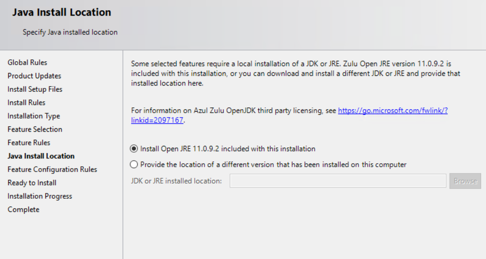
When installing a new instance of SQL 2019 or adding the Polybase feature to an existing installation of SQL 2019 you will go through the installation wizard until you get to this page:

As you can see, you’re now prompted to either Install Open JRE 11.0.3 included with this installation (default). Or to specify the location of your other JRE/JDK installation.

Problem:

Let’s suppose that you installed SQL 2016 with Polybase, had installed and ran on Oracle JRE 8 but after Oracle’s 2018 announcement decided that you needed to upgrade to SQL 2019 and switch to using Azul Open JRE. You’ve already uninstalled Oracle JRE but when you go to upgrade to SQL 2019 there is no option for selecting a different JRE version. What do you do?

Solution:

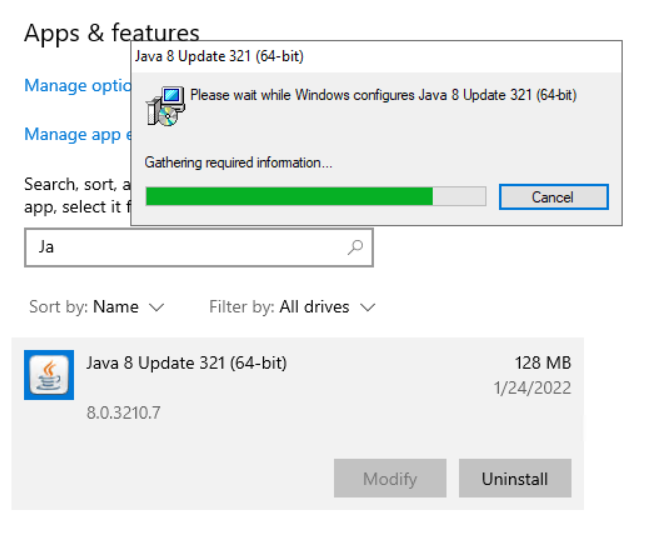
Before you start the upgrade to SQL 2016, make sure that you uninstall Java JRE 8 from the server. You can do this easily through the regular add/remove programs:

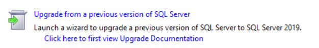
Next go ahead and launch the SQL 2019 installation media and proceed as normal through the Upgrade wizard:

Upgrade from a previous version of SQL Server

Select your instance and continue:

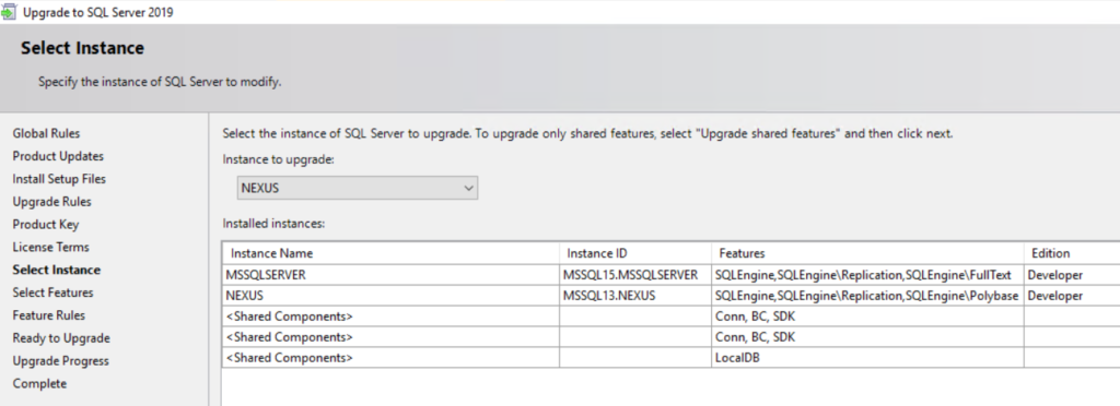
While going through the wizard, you will notice the absence of any option to specify the JRE version or path. That’s ok and what you should expect to see.

Continue through the upgrade wizard to completion.

After the installation completes check the registry at: Computer\HKEY_LOCAL_MACHINE\SOFTWARE\Microsoft\Microsoft SQL Server\MSSQL15.MSSQLSERVER\Polybase\Configuration

The JavaInstalledLocation key should not be present. If it is present that means that you forgot to uninstall the Oracle Java JRE. If you did, that’s ok just go ahead and uninstall it now then check the registry key again after rebooting.

If the key is still present after rebooting then go ahead and delete it.

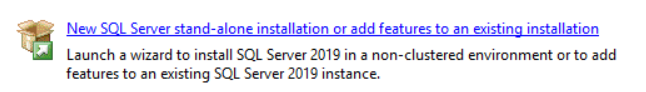
Finally, relaunch the SQL 2019 Installation Center and select add features to an existing installation:

Installation Center: New SQL Server stand-alone installation or add features to an existing installation

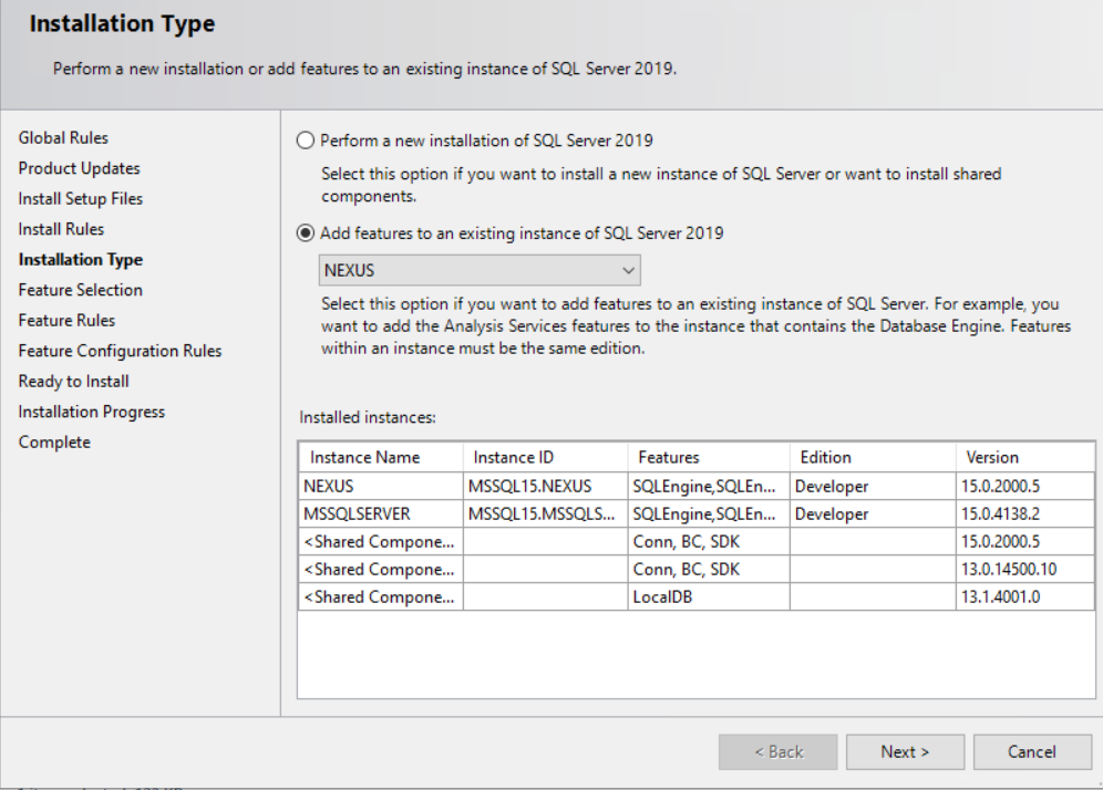
On the “Installation Type” step of the wizard, select the instance with Polybase that you just upgraded to SQL 2019.

Installation Type: Add features to an existing instance of SQL Server 2019

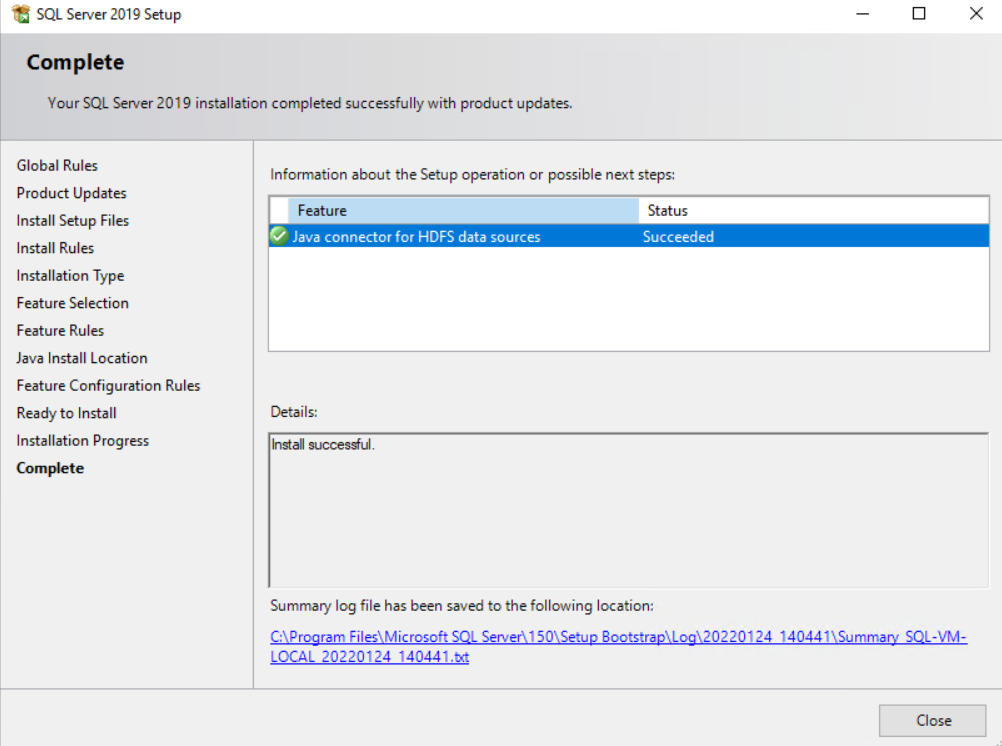
On the next step of the wizard Feature Selection, scroll down and you should see the PolyBase Query Service for External Data box is already checked and greyed out. But there is a new box nested underneath labeled Java connector for HDFS data sources:

Feature Selection: Java connector for HDFS data sources

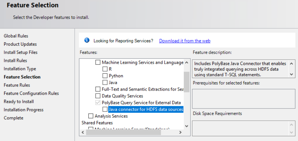
Check this box and click next.

On the next screen you will now have the option to Install Open JRE 11.0.9.2 (default) or to Provide the location of a different version that has been installed on this computer.

Complete the rest of the steps of the installation and it should install successfully.

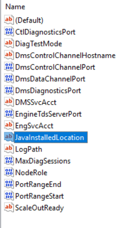
To verify that the desired Java JRE is being used by SQL Server Polybase, open up the registry again and navigate to: Computer\HKEY_LOCAL_MACHINE\SOFTWARE\Microsoft\Microsoft SQL Server\MSSQL15.NEXUS\Polybase\Configuration

You should now see the JavaInstalledLocation key:

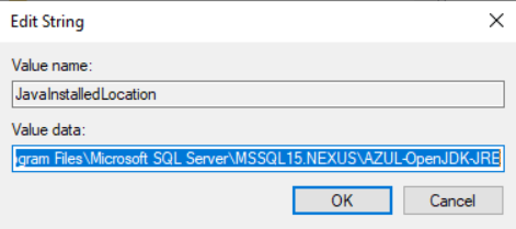
If you click modify you should see that the value is the path of the Java installation you selected or if using Azul JRE, something like this:

C:\Program Files\Microsoft SQL Server\MSSQL15.NEXUS\AZUL-OpenJDK-JRE

I personally tested these steps on SQL Server 2016 but the same steps should work on an upgrade from SQL 2017 to 2019.

Data Structures: Queue

A Queue is a FIFO (First In First Out — the element placed at first can be accessed at first) structure which can be commonly found in many programming languages. This structure is named as “queue” because it resembles a real-world queue — people waiting in a queue (line).

Just like in like real life, the person who was in line first gets served first.

Queue Operations

Given below are the 2 basic operations that can be performed on a queue. Reference the diagram above

Enqueue: Insert an element to the end of the queue.
Dequeue: Delete the element from the beginning of the queue.

Applications of Queues

Used to manage threads in multithreading.
Used to implement queuing systems (e.g.: priority queues).

Data Structures: Stack

A Stack is a linear data structure which follows a particular order in which the operations are performed. The order may be LIFO (Last In First Out) or FILO (First In Last Out).

Push: Insert an element on to the top of the stack.

Pop: Delete the topmost element and return it.

Furthermore, the following additional functions are provided for a stack in order to check its status.

Peek: Return the top element of the stack without deleting it.
isEmpty: Check if the stack is empty.
isFull: Check if the stack is full.

Applications of stacks

Used for expression evaluation (e.g.: shunting-yard algorithm for parsing and evaluating mathematical expressions).
Used to implement function calls in recursion programming.

Data Structures: Array

An array is a collection of items stored at contiguous memory locations. The idea is to store multiple items of the same type together. This makes it easier to calculate the position of each element by simply adding an offset to a base value, i.e., the memory location of the first element of the array.

The diagram above demonstrates how each element can be uniquely identified by its index value or by its memory address. Notice that the memory addresses are sequential. This is what is meant by contiguous (touching). This demonstrates how and why order is preserved with arrays.

Data Structures: Doubly Linked List

A Doubly Linked List (DLL) is very similar to a Linked List, but contains an extra pointer, typically referred to as previous pointer, together with next pointer and the data.

Advantages over singly linked list

A doubly linked list can be traversed in both forward and backward direction.
The delete operation for doubly linked lists is more efficient if pointer to the node to be deleted can be supplied.
Quickly insert a new node before a given node.
In a singly linked list, to delete a node, the pointer to the previous node is needed. To get the previous node, the list has to be traversed from the beginning. Whereas the doubly linked list can fetch the previous node using previous pointer.

DisadvantageS

Every node of the doubly linked list requires extra space for the previous pointer.
All operations have additional overhead because of the extra previous pointer. For example, in insertion, we need to modify previous pointers together with next pointers.

Insertion

A node can be added in four ways:

At the front of the DLL
After a given node.
At the end of the DLL
Before a given node.

Data Structures: Linked List

Like arrays, the Linked List is a linear data structure. Unlike arrays, linked list elements are not stored at a contiguous location; the elements are linked using pointers.

Like arrays, the Linked List is a linear data structure. Unlike arrays, linked list elements are not stored at a contiguous location; the elements are linked using pointers.

Why use a Linked List over an Array?

Arrays can be used to store linear data of similar types, but arrays have the following limitations:
1) Arrays have a fixed size – so we must know the upper limit (ceiling) on the number of elements in advance. Additionally, in most implementations, the memory allocation is equal to the upper limit regardless of usage.
2) Inserting new elements into an array is expensive because space has to be created for the new elements and to create space, existing elements have to be shifted.
For example, in a system, if we maintain a sorted list of IDs in an array nums[].
nums[] = [100, 101, 105, 200, 206].
And if we want to insert a new ID 104, then to maintain the sorted order, we have to move all the elements after 100 (excluding 100).
Deletion is also expensive with arrays. For example, to delete 101 in nums[], everything after 101 has to be shifted.

Advantages over arrays:

Dynamic size
Ease of insertion/deletion

Disadvantages:

Random access is disallowed. We must access elements sequentially starting from the first node and then traverse the list until we reach the element we are seeking. So an efficient binary search is not an option with linked lists in their default implementation.
The more segments a list is broken into the more overhead there is for locating the next linked element.
Extra memory space for a pointer is required with each element of the list.
Not cache friendly. Since array elements are contiguous locations, there is locality of reference which is not the case for linked lists.

Representation

A linked list is represented by a pointer to the first node of the linked list. The first node is called the head. If the linked list is empty, then the value of the head is NULL.
Each node in a list consists of at least two parts:
1) Data
2) Pointer (Or Reference) to the next node

MSSQL Server: Always On AG Synchronous Commit is NOT Synchronous Redo

Microsoft SQL Server Always On Availability Groups was introduced in SQL Server 2012 and were a more mature, stable and robust version of database mirroring. In fact, the AG feature was built with mirroring at its foundation. SQL Server 2014 introduced several improvements including increasing the readable secondaries count and sustaining read operations upon secondary-primary disconnections, and it provides new hybrid disaster recovery and backup solutions with Microsoft Azure.

As the feature became more mature and stable I began seeing environments that really pushed the limits of what the technology was capable of.

Always On AG Data Synchronization Flow

Sequence	Step	Description
1	Log generation	Log data is flushed to disk. This log must be replicated to the secondary replicas. The log records enter the send queue.
2	Capture	Logs for each database is captured and sent to the corresponding partner queue (one per database-replica pair). This capture process runs continuously as long as the availability replica is connected and data movement is not suspended for any reason, and the database-replica pair is shown to be either Synchronizing or Synchronized. If the capture process is not able to scan and enqueue the messages fast enough, the log send queue builds up.
3	Send	The messages in each database-replica queue is dequeued and sent across the wire to the respective secondary replica.
4	Receive and cache	Each secondary replica receives and caches the message.
5	Harden	Log is flushed on the secondary replica for hardening. After the log flush, an acknowledgment is sent back to the primary replica. Once the log is hardened, data loss is avoided.
6	Redo	Redo the flushed pages on the secondary replica. Pages are kept in the redo queue as they wait to be redone.

Source: Monitor performance for availability groups – SQL Server Always On | Microsoft Docs

The diagram above demonstrates the data movement steps for a simple two node Always On AG with Synchronous Commit Enabled.

Put briefly, a transaction occurs on the Primary and waits (logged as HADR_SYNC_COMMIT waits) while the transaction is sent across the wire to the Secondary replica. The secondary replica hardens the transaction to the log then sends an acknowledgement back to the Primary. Having received confirmation from the secondary that the data is safely committed to the transaction log, the primary can now issue a commit to finish its own transaction and release any locks it may have been holding.

But wait… when exactly does redo occur? Notice that step 6 which involves the redo process is purposefully separated from the rest of the data flow. This is because even when the AG is set to Synchronous Commit, the Redo still occurs asynchronously.

Asynchronous Redo: Potential Impact From Long Failovers and Extended Recovery

Synchronous Commit is a configuration option for Availability Groups but in my opinion it is really more of a Disaster Recovery feature than a High Availability Feature because it’s primary function is to make sure that in the even of a failure of the primary node, failover to a secondary node can occur either manually or automatically with zero data loss (Disaster Recovery) but no guarantees are made about how long it takes to perform the failover (High Availability).

Because we do not commit on the primary until the transaction hardens on the primary, data consistency is guaranteed. However, since changes are applied to the data file from the redo queue on the secondary with no synchronization mechanism to prevent the primary from “getting ahead”, it is possible for the data on the secondaries to lag behind. When this occurs you will see the redo queue grow in size and failovers may take longer than expected. This is because during a failover the secondary database is brought from a Restoring/Synchronizing state to an Online state. Part of the onlining process is the three Recovery steps:

Phase 1: Analysis
Phase 2: Redo
Phase 3: Undo

That’s right, as part of the failover all of the transactions that had been committed but not yet redone must now be redone before the database can come online. The same is true if there is no failover but the local instance is in the Primary role and restarts. This becomes especially burdensome if there are a high number of VLFs which likely means the not yet redone transactions are also heavily fragmented.

Asynchronous Redo: Potential Impact to Readable Secondaries

In addition to impacting failover recovery intervals, there is the potential to impact read-only data consistency. Now that sounds bad, but in my experience the scenario is quite rare. Basically, the issue manifests itself if you have an workflow that performs a DML operation on the primary and then IMMEDIATELY check for the updated row on the secondary. In this scenario it is possible that the transaction has been committed on the primary and hardened to the secondary’s log but not yet redone – leading to what appears to be inconsistent data.

So why not have synchronous redo too? Well, to understand that you need to be familiar with CAP Theorem which basically states you can’t have it all. Between high availability, partitioning and consistency you can only pick two. Now, with synchronous commit mode we are already sacrificing consistency because of the brief time between harden and redo. However, if we wanted to keep redo on the secondary in sync with data writes on the primary one of two things would have to happen:

The transaction is hardened and then instantaneously written to the data file (impossible).
The data modification on the primary is postponed until the change is redone on the secondary.

While the second option is technically possible but it would have a detrimental impact to performance (think about the impact HADR_SYNC_COMMIT waits can have but worse). The only way for it not to impact performance would be if we let the transaction commit and release its locks then lazily applied the change to the data file afterwards. This would be bad for many reasons but imagine for instance that your transaction is a bank transaction. You initiate a transfer of your entire balance, the transaction commits and sends a confirmation back, then you go to immediately initiate another transfer which should be disallowed but under a synchronous redo scenario that sacrifices consistency for performance, the balance would not have been updated yet despite the transaction committing.

So, in summary, the reason there is no Synchronous Redo for Always On AGs because it would be detrimental to performance and/or would violate ACID Principles.

MSSQL Server: Always On AG RegisterAllProvidersIP & MultiSubnetFailover=True

The Microsoft SQL Server Always On Availability Groups feature is often confused with the similarly named SQL Server Always On Failover Cluster instances. This is in part because Failover Cluster Instances (FCI) were rebranded some years ago under the “Always On” marketing term, but also because both features rely on the Windows Failover Cluster feature. In this article I will exclusively be talking about the availability group feature and may abbreviate it as Always On AG or just simply AG.

Note
Always On availability groups is the full, formal name for this availability feature. The abbreviation is AG, not AOAG or AAG.
Microsoft Always On availability groups: a high-availability and disaster-recovery solution

Multi-subnet Clusters

A SQL Server multi-subnet failover cluster is a configuration where each failover cluster node is connected to a different subnet or different set of subnets. There are many reasons why you may want to have a multi-subnetted cluster (or are forced to use one) including geographically dispersed sites.

When an AG is built on a Windows Server Failover Cluster (WSFC) that spans multiple subnets, a properly configured Always On AG Listener will have an IP address for each defined subnet and each will have an OR dependency in the Cluster Manager. By default, when the Listener is added, it gets registered in DNS by the Windows Cluster. The cluster will submit all of the IP addresses in the dependency list and the DNS server will register an A record for each IP address.

When a client tries to connect to the AG using the Listener name, the DNS server gets queried and all of the A records are returned. The cluster resource for the IP that is a member of the subnet for which the primary replica node of the AG is currently hosted will be online while all the other cluster resource IPs will be offline. Depending on the client, this can cause problems.

Timeout Problems

The default behavior of most supported SQL Client connectivity drivers is to try each one of the IP addresses in DNS associated with the Listener one-by-one (serially). This happens in the following order:

Client initiates connection with Listener name specified in connection string
Query DNS for the listener name
DNS returns IP addresses of all A records matching the Listener name (in an indeterminate order)
Client tries to connect to listener using the first IP returned
Client times out after the TCP connection attempt timeout (default 21 seconds)
If the previous connection attempt times out, attempt using the next IP address

So what is the problem? Well, the problem is that while the TCP connection timeout is 21 seconds, the default .NET client application timeout value is 15 seconds. When the application times out, the whole connection closes.

So if you have a client configured with the default timeout value, and you don’t get lucky with the first IP returned by DNS, you’ll never make it far enough to try the rest of the IPs. This often times does not manifest itself as a problem until the first time you try to failover production and manifests itself as repeated connection timeouts from your client applications trying to connect to SQL Server until you fail back to the original node. So what can you do?

Resolution: MultiSubnetFailover=True

The good news is that if you’re using at least SQL Server 2012 and your .NET application is on at least .NET 4.5 (earlier .NET libraries with hotfixes), you can take advantage of the new connection parameter that Microsoft added, MultiSubnetFailover, which should be used and set to TRUE. This changes the serial connection attempt behavior mentioned prior to what is essentially parallel connection attempts¹.

Now, when you try to connect to SQL using the Listener, even if there are multiple A records, your application will try them all at once instead of one-by-one lessening the chances of a timeout.

Workaround: Older or Incompatible Clients

In a perfect world we’d just upgrade everything all the time seamlessly, immediately and without impacting the business’s bottom line. However, in reality, legacy applications exist. If you find yourself in a scenario where setting MultiSubnetFailover=True is not an option for at least one of your applications, you’ll need a work around.

Assuming that your organization is using Dynamic DNS, one option may be to modify the RegisterAllProvidersIP cluster setting. This parameter determines whether the Windows Cluster will register all of the IP addresses for the AG Listener, or only the one for the one currently online in the Cluster Manager (so the one that is a member of the subnet where the AG primary is). When set to 1(default if the AG Listener is created by SQL Server²), the AG Listener clustered resource gets created with all of the IP addresses.

With the cluster reconfigured to only register only one A record in DNS at a time, this introduces another potential issue: an outdated DNS. with default TTL on the A record, the failover has a high probability of completing much more quickly than DNS gets updated with the new IP address. This means that even after a failover your clients could still get timeout errors because the Listener A record is still pointing to the secondary node post failover. This will eventually resolve itself once the TTL expires but that may be long after your business’s SLAs. To mitigate the effects of this, we can use the HostRecordTTL cluster parameter. This parameter governs how long (in seconds) before cached DNS entries on a client OS are expired, forcing the client OS to re-query the DNS server again to obtain the current IP address. By default, this value is 1200 (20 minutes). 20 minutes is a really long time to potentially wait before clients can successfully connect again after a failover. To ensure that we can connect sooner, we should set this to something like 120 or 60.

The drawback to setting the value to a lower number is how often the client OS will query the DNS server. If you have a handful of application servers, then changing the value from 1200 to 60 would probably have no perceptible impact on the DNS server(s). However, if there are thousands of client machines that all must resolve the AG Listener name to IP, this increases the load on the DNS server(s) and could cause problems.

You will need to strike a balance between the lowest possible cache expiration time and the increased overhead for the DNS server.

¹All IP addresses receive a SYN request at the TCP layer and are rapidly initiated one-by-one (so still serially) but do wait for acknowledgement before initiating the next connection attempt (so close enough to parallel for the purposes of this article).
²If a Client Access Point is created using Windows Failover Cluster Manager, the RegisterAllProvidersIP parameter is set to 0 by default.

MSSQL: Database Mail – Failed to initialize sqlcmd library with error number -2147467259

This is a common error and most search results on the web point out the most common cause for this error (which is also documented in the official Microsoft documentation):

The following error may occur when setting @query_result_header to 0 and setting @query_no_truncate to 1:
Msg 22050, Level 16, State 1, Line 12: Failed to initialize sqlcmd library with error number -2147024809.
Microsoft: sp_send_dbmail (Transact-SQL)

However, I recently came across another scenario that can cause [almost]* the exact same error and leave you scratching your head over something that is really just a simple mistake.

*If you look closely the Msg number is the same but the error number is different: -2147467259 vs -2147024809

Scenario

I enabled database mail and tried to execute the following query:

EXEC msdb.dbo.sp_send_dbmail
	@profile_name= 'dbamail',
	@recipients = '[email protected]',
	@subject = 'Test',
	@body = 'File attached',
	@query = 'select count(*) from dbo.members;',
	@attach_query_result_as_file = 1, 
	@query_attachment_filename = 'MemberCount.csv';

And got the following error:

Msg 22050, Level 16, State 1, Line 12: Failed to initialize sqlcmd library with error number -2147467259.

Like everyone else I searched online, came across the blog posts as well as the official Microsoft documentation and added the appropriate parameters (even though they should have been the defaults since I did not explicitly set them before).

EXEC msdb.dbo.sp_send_dbmail
	@profile_name= 'dbamail',
	@recipients = '[email protected]',
	@subject = 'Test',
	@body = 'File attached',
	@query = 'select count(*) from dbo.members;',
	@attach_query_result_as_file = 1, 
	@query_attachment_filename = 'MemberCount.csv',
	@query_result_header = 1, @query_no_truncate = 0

But got the same error:

Msg 22050, Level 16, State 1, Line 12: Failed to initialize sqlcmd library with error number -2147467259.

Solution:

If you look at my code you’ll notice that there is an optional parameter not specified: @execute_query_database

[ @execute_query_database = ] 'execute_query_database' Is the database context within which the stored procedure runs the query. The parameter is of type sysname, with a default of the current database. This parameter is only applicable if @query is specified.
Microsoft: sp_send_dbmail (Transact-SQL)

I’d like to point out the line that says “with a default of the current database” because when I checked I had forgotten to change the current database context in SSMS to my user database instead of master. However, when I changed the context to my user database it was still failing with the same error.

I couldn’t successfully send my databasemail with attachment until I specified this parameter explicitly:

EXEC msdb.dbo.sp_send_dbmail
	@profile_name= 'dbamail',
	@recipients = '[email protected]',
	@subject = 'Test',
	@body = 'File attached',
	@execute_query_database = 'myDB',
	@query = 'select count(*) from dbo.members;',
	@attach_query_result_as_file = 1, 
	@query_attachment_filename = 'MemberCount.csv',
	@query_result_header = 1, @query_no_truncate = 0;

Specifying the database name in the bindings of my select query also seemed to work:

EXEC msdb.dbo.sp_send_dbmail
	@profile_name= 'dbamail',
	@recipients = '[email protected]',
	@subject = 'Test',
	@body = 'File attached',
	@query = 'select count(*) from myDB.dbo.members;',
	@attach_query_result_as_file = 1, 
	@query_attachment_filename = 'MemberCount.csv',
	@query_result_header = 1, @query_no_truncate = 0;

Conclusions

My philosophy is to be as verbose as possible if doing so doesn’t increase the complexity of the problem you are trying to solve. In this case I shouldn’t have relied on MSSQL Server or SSMS to predict the database I was trying to execute against.

SSMS can also be unreliable for these types of things because of the way it asynchronously changes or updates it’s GUI. My suspicion is that even though I changed the database context with the drop down menu, I never clicked back into the query editor window and so the session wasn’t updated. I could have gone back and tested this theory but it seemed moot point since the best solution is obviously to just specify the database in my query.

Bitwise Operations

Human readable code is certainly not the point.

What is Bitwise Manipulation?

Bitwise manipulation is when we perform a logical operation against each individual bit of a binary number. The logical connectives a.k.a. the bitwise operators AND, OR, and XOR can be used as masks that can affect the specific bits.

What is the point of Bitwise manipulation?

Human readability is certainly not the point, but speed and efficiency are. Bitwise operations are primitive actions that can be executed directly on the CPU meaning that they stake up less temporary/persistent storage and require less pre-processing overhead to compute. You can think of them like shortcuts.

AND

The AND logical operation can be used to turn off certain bits of a binary number, because:

1 AND 0 is 0

0 AND 0 is 0

Consider you have an input of 1101 1011 and a bitwise mask of 1111 1000. Examine the function table below:

Input	1	1	0	1	1	1	1
Mask	1	1	1	1	1	0	0
Result	1	1	0	1	1	0	0

Bitwise AND Mask Results

Notice that the mask only applies to the last three digits. The third to last digit is unchanged only because it was already 0.

OR

The AND logical operation can be used to turn off certain bits of a binary number, because:

1 AND 0 is 0

0 AND 0 is 0

Consider you have an input of 1001 1011 and a bitwise mask of 1110 0000. Examine the function table below:

Input	1	0	0	1	1	1	1
Mask	1	1	1	0	0	0	0
Result	1	1	1	1	1	1	1

Bitwise OR Mask Results

Notice that only the first three digits changed (except the first digit which was already a 1). The OR switch changed all the 0 bits to 1’s.

XOR

The XOR (Exlusive OR) logical function can be used to reverse certain bits of a binary number, because:

0 XOR 1 is 1

1 XOR 1 is 0

Consider you have an input of 1011 1001 and a bitwise mask of 0000 1111. Examine the function table below:

Input	1	1	1	1	0	0	1
Mask	0	0	0	1	1	1	1
Result	1	1	1	0	1	1	0

Bitwise XOR Mask Results

Notice that all four of the bits aligned with the mask are now the opposite of what they once were without exceptions. The bits have essentially been “flipped”.

Logical Shift Left

Performing a logical shift one bit to the left on a binary number means:

Moving all the bits of the number one place to the left
Discarding the most significant bit
Putting a 0 into the empty place on the right

Interestingly this is equivalent to multiply our binary number by 2. Notice that performing a logical shift three bits to the left on a binary number is the same as multiplying the number by 2³= 8.

Example:

If we start with the decimal number 14, three logical shifts to the left of its binary form results in the decimal number 112:

	128	64	32	16	8	4	2	1
14₁₀	0	0	0	0	1	1	1	0
28₁₀	0	0	0	1	1	1	0	0
56₁₀	0	0	1	1	1	0	0	0
112₁₀	0	1	1	1	0	0	0	0

Logical Shift Left Results

Logical Shift Right

Performing a logical shift one bit to the right on a binary number means:

Moving all the bits of the number one place to the right
Discarding the least significant bit
Putting a 0 into the empty place on the left

As you might have guessed, this is equivalent to dividing our number by 2. Notice that performing a logical shift two bits to the right on a binary number is the same as dividing the number by 2² = 4.

Example:

If we start with the decimal number 112, two logical shifts to the right of its binary form results in the decimal number 28:

	128	64	32	16	8	4	2	1
112₁₀	0	1	1	1	0	0	0	0
56₁₀	0	0	1	1	1	0	0	0
28₁₀	0	0	0	1	1	1	0	0

Logical Shift Right Results